cells_path <- here::here("data/cells.csv")
pines_path <- here::here("data/black_pines.csv")
redwoods_path <- here::here("data/redwood_seedlings.csv")

cells <- readr::read_csv(cells_path, show_col_types = FALSE)
pines <- readr::read_csv(pines_path, show_col_types = FALSE)
redwoods <- readr::read_csv(redwoods_path, show_col_types = FALSE)Exploring Point Processes
Workshop 1: The Poisson Process
Session Outline
- Recap
- The Poisson Process
- Formal Definitions
- Useful Properties & Areas for Further Exploration
Recap: What is a Point Process?
Defining a Point Process
A point process is a stochastic process where:
RVs \(\{X_1, \ldots, X_N\}\) represent localised events on some (typically continuous) mathematical space \(S\).
We are interested in value and number of events, but both of these are random.
Events \(X \in S\) vs. points / locations \(s \in S\).
Example: Temporal point process
Example: 1D point process
Example: 2D point process
The Homogeneous Poisson Process
Number of events is Poisson distributed, \(N \sim \text{Pois}(\lambda |S|)\).
Events located independently of one another, uniformly at random over \(S\).
In the 2D context, this is known as complete spatial randomness.
HPP as a central case


Trying to reference Figure 1.
Visual Assessment of CSR
Some simulated point patterns - which is random, clustered or repulsive?


HPP as a null model
- Interesting theoretical properties, see some soon.
- Too simple to be a useful model, but a good starting point.
- Use as a null model - analogous to regression.
- Identify shortcomings as a starting point for further exploration.
Definitions of a Poisson Process
Recap: many interpretations of the same process
\[ \mathcal{X} = \{(X_1,X_2)^T\}, \quad X \sim \text{MVN} \left(\mathbf{\mu}, \Sigma \right). \]
Or
\[ \mathcal{X} = \{(X_1,X_2)^T\},\]
where
\[ X_1 \sim \mathcal{N}(\mu, \sigma^2), \\ X_2|X_1=x_1 \sim \mathcal{N}\left(\mu_2 + \frac{\sigma_2\rho(x_1 - \mu_1)}{\sigma_1}\ , \ (1 - \rho^2)\sigma_2^2 \right).\]
Recap: many interpretations of the same process
HPP as limit of Binomial Process
Working in continuous time or space is hard. Start discrete and consider the limit
\[\begin{equation*} \{X_1, \ldots, X_m\} \overset{\perp}{\sim} \text{Bern}(p_i). \end{equation*}\]
For now we will let \(p_1 = p_2 = \ldots = p\),
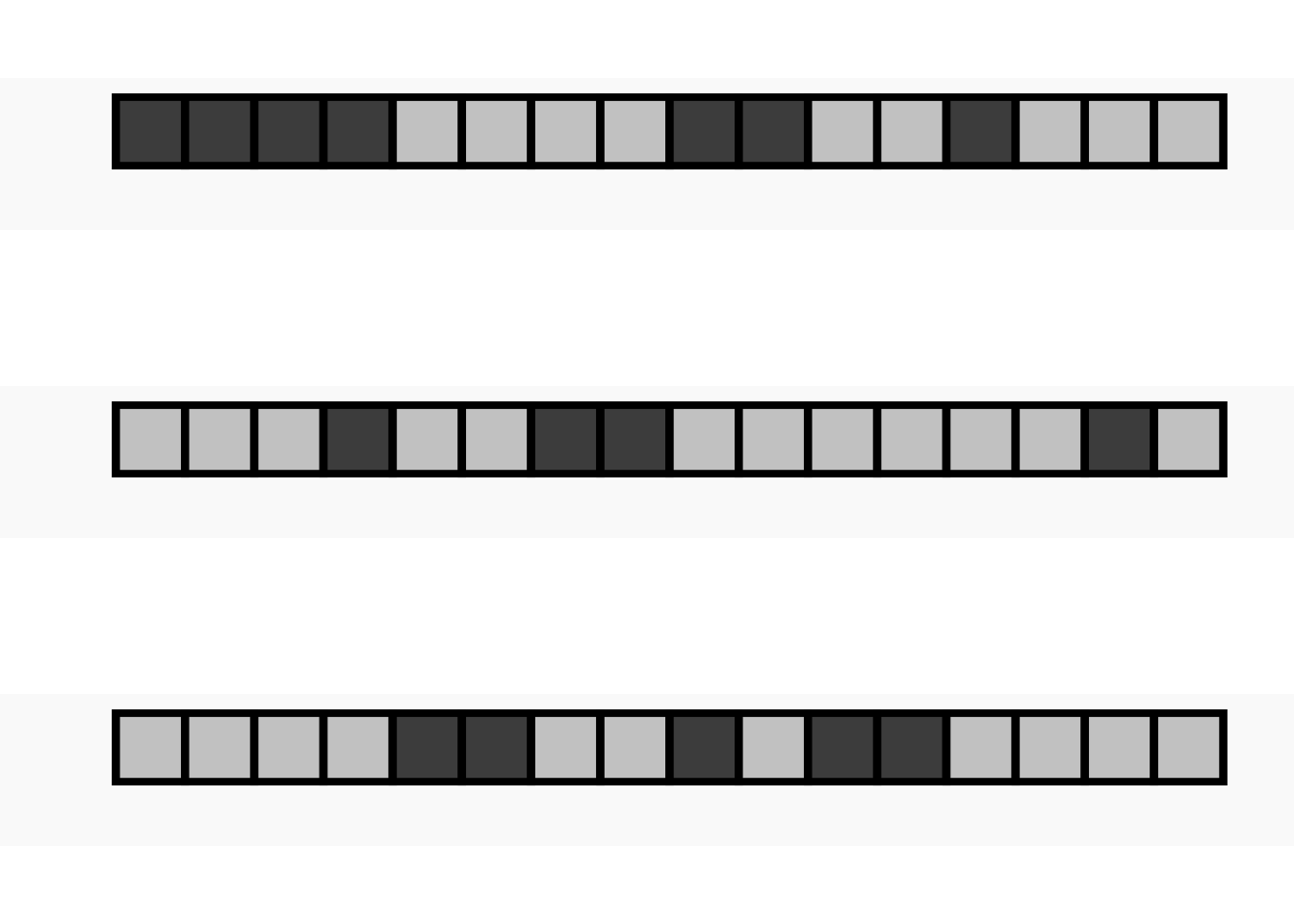
The total number of events in the process:
\[\begin{equation*} N = \sum_{i=1}^{m} X_i \sim \text{Binom}(m , p). \end{equation*}\]
So
\[\begin{equation*} \mathbb{E}[N] = m p, \quad \text{Var}(N) = m p (1-p) \end{equation*}\]
and for \(A \subseteq S\), \(N(A) \sim \text{Binom}\left(\frac{|A|}{|S|}m, p\right).\)
Code
# histogram ----------

hist_df <- tibble(
n = seq(0, 25),
pdf = dbinom(n, size = 25, prob = 0.3)
)

p_hist <- ggplot(data = hist_df, mapping = aes(x = n, y = pdf)) +
  geom_col() +
  ylab("Pr(N = n)") +
  zvplot::theme_zv()

# grid ----------------
n <- 5
p <- 0.3

grid_df <- tibble(
  x = rep(1:n, times = n),
  y = rep(1:n, each = n),
  z = rbinom(n = n * n, size = 1, prob = p),
  fill_col = if_else(as.logical(z), "grey30", "grey80")
)

p_grid_5 <- ggplot(data = grid_df, aes(x = x, y = y)) +
  geom_tile(aes(fill = fill_col), col = "black", lwd = 1.5) +
  scale_fill_identity() +
  coord_fixed() +
  ylab("") +
  xlab("") +
  zvplot::theme_zv()

print(p_hist)
print(p_grid_5)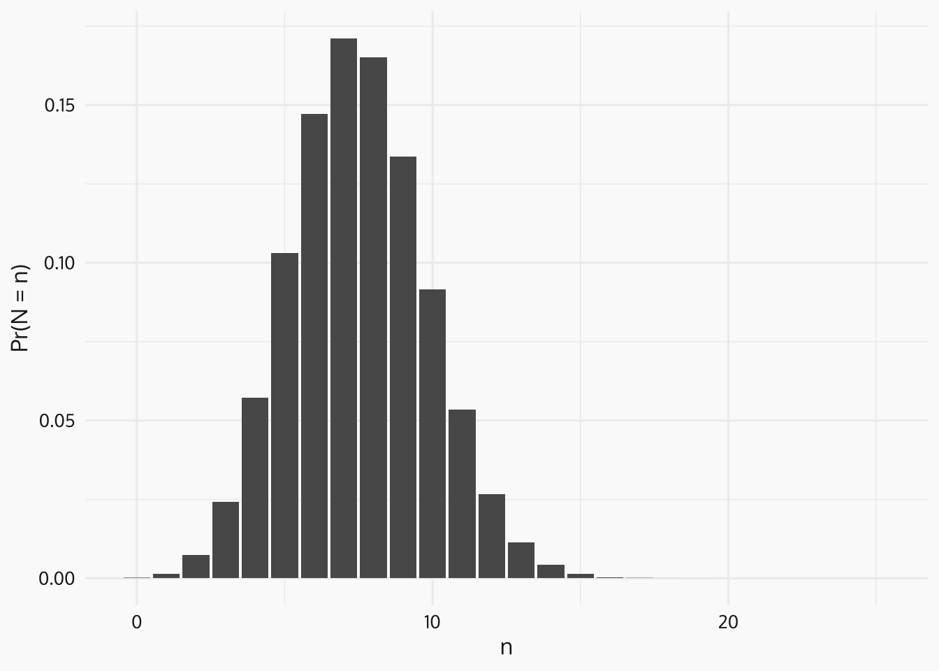
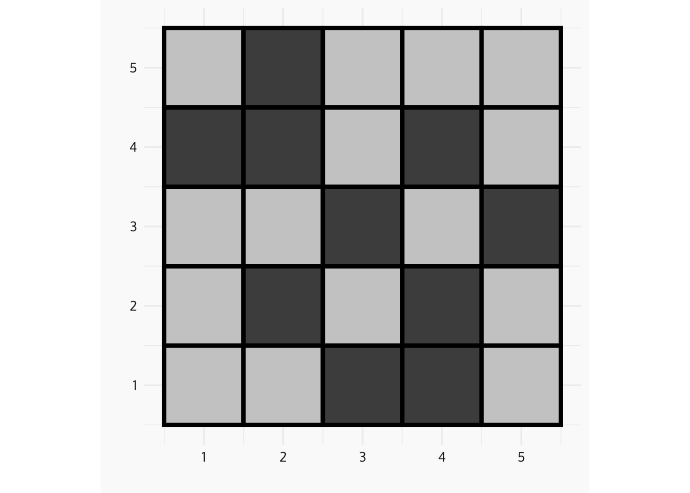
HPP as limit of Binomial Process - Increase the Resolution
Code
n <- 10
p <- 0.3 * (5/n)^2

grid_df <- tibble(
  x = rep(1:n, times = n),
  y = rep(1:n, each = n),
  z = rbinom(n = n * n, size = 1, prob = p),
  fill_col = if_else(as.logical(z), "grey30", "grey80")
)

p_grid_10 <- ggplot(data = grid_df, aes(x = x, y = y)) +
  geom_tile(aes(fill = fill_col), col = "black", lwd = 1.5) +
  scale_fill_identity() +
  coord_fixed() +
  ylab("") +
  xlab("") +
  zvplot::theme_zv() +
  theme(axis.text = element_blank())

print(p_grid_10)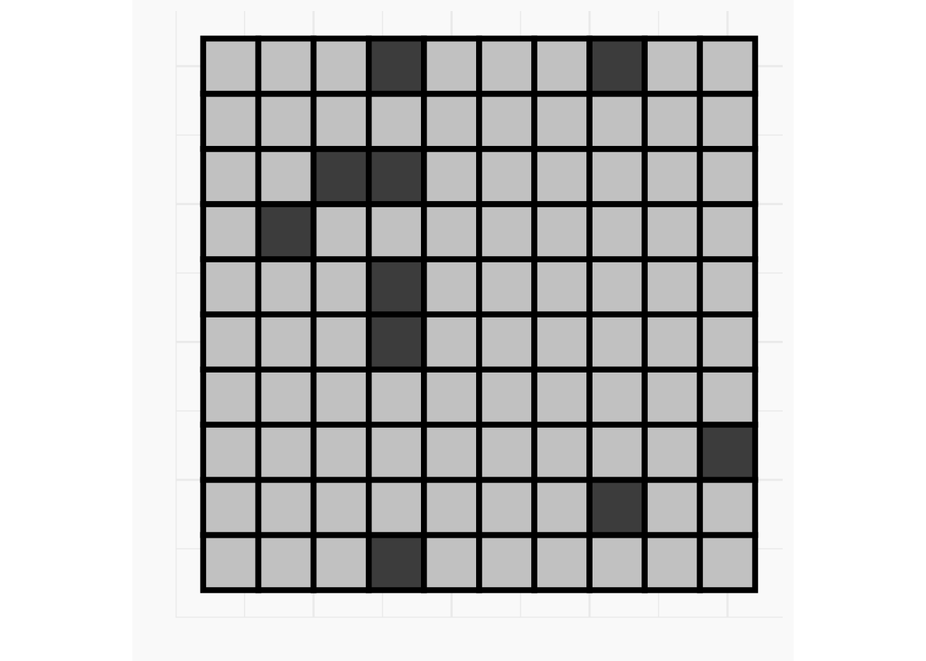
Code
n <- 20
p <- 0.3 * (5/n)^2

grid_df <- tibble(
  x = rep(1:n, times = n),
  y = rep(1:n, each = n),
  z = rbinom(n = n * n, size = 1, prob = p),
  fill_col = if_else(as.logical(z), "grey30", "grey80")
)

p_grid_20 <- ggplot(data = grid_df, aes(x = x, y = y)) +
  geom_tile(aes(fill = fill_col), col = "black", lwd = 1) +
  scale_fill_identity() +
  coord_fixed() +
  ylab("") +
  xlab("") +
  zvplot::theme_zv() +
  theme(axis.text = element_blank())

print(p_grid_20)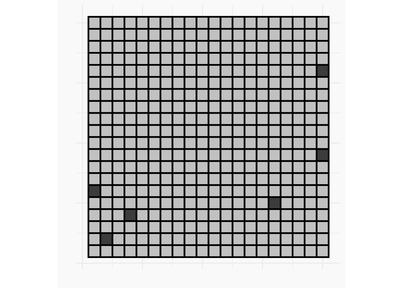
Code
n <- 100
p <- 0.3 * (5 / n)^2

grid_df <- tibble(
  x = rep(1:n, times = n),
  y = rep(1:n, each = n),
  z = rbinom(n = n * n, size = 1, prob = p),
  fill_col = if_else(as.logical(z), "grey30", "grey80")
)

p_grid_100 <- ggplot(data = grid_df, aes(x = x, y = y)) +
  geom_tile(aes(fill = fill_col)) +
  scale_fill_identity() +
  coord_fixed() +
  ylab("") +
  xlab("") +
  zvplot::theme_zv() +
  theme(axis.text = element_blank())

print(p_grid_100)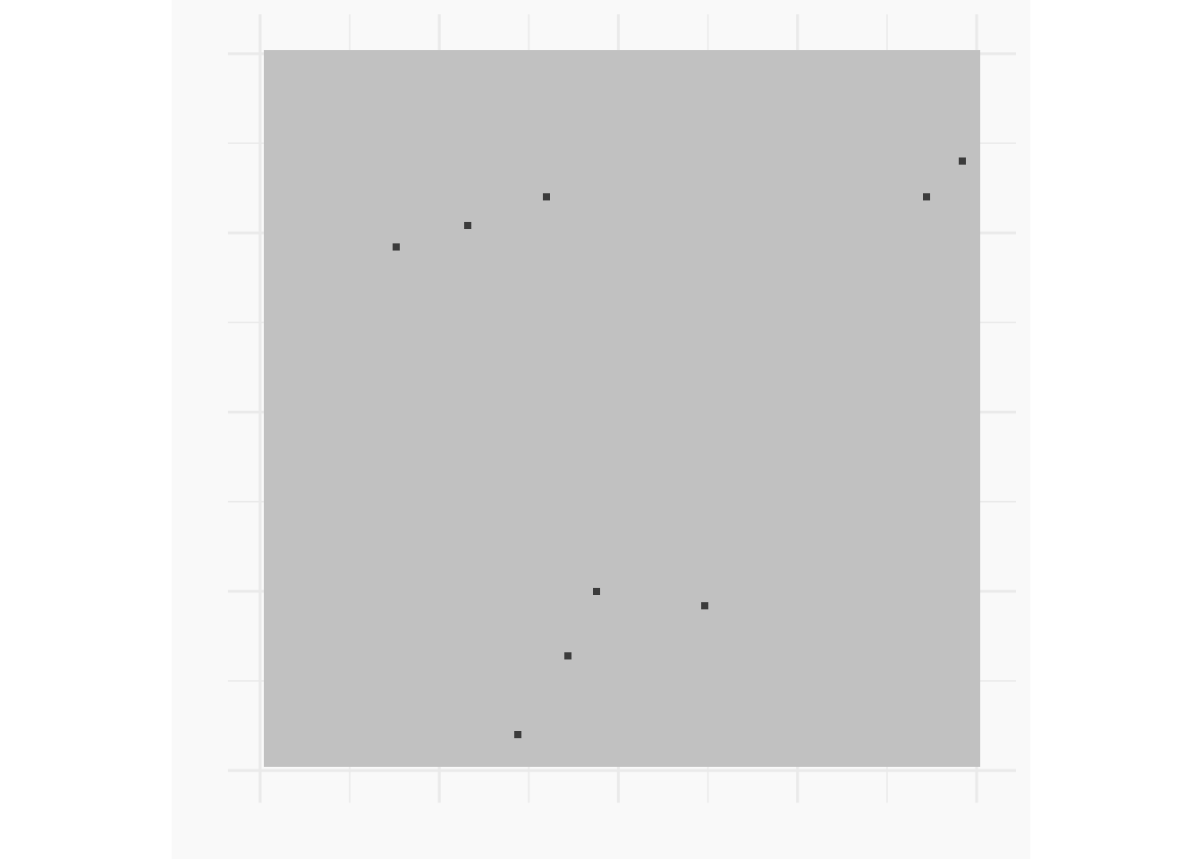
Looking at the limit: counting specification
Each time we increase the resolution by a factor of \(k\) we get more events (in expectation). To keep this constant, we divide \(p\) by an appropriate multiplier.
Formally, let \(m \rightarrow \infty\) and \(p \rightarrow 0\) such that \(m p \rightarrow \lambda \in \mathbb{R}^+\). Then
\[\begin{equation*} N(A) \overset{D}{\rightarrow} \text{Pois}(\lambda) \quad \text{ and } \quad N(A) \perp N(B) \text{ when } A \cap B = \emptyset. \end{equation*}\]
This is the counting specification of an HPP.
Inhomogeneous PP and the intensity specification
Generalise by no longer assuming that \(p_1 = \ldots = p_m = p\).
\(N(A) = \sum_{i \in A} X_i\) so \(\Pr(N(A) = n) = \Pr(\sum_{\{i \ :\ a_i \in A\}} X_i = n)\) and:
\[\begin{equation*} \mathbb{E}[N(A)] = \sum_{i=1}^{m} p_i \ \mathbb{I}(a_i \in A), \end{equation*}\]
\[\begin{equation*} \text{Var}(N(A)) = \sum_{i=1}^{m} p_i (1 - p_i) \ \mathbb{I}(a_i \in A). \end{equation*}\]
Introducing the intensity function
Describe the local rate of events by the intensity function:
\[\begin{equation*} \lambda(s) = \lim\left(\frac{ N(s, s+\delta)}{\delta}\right) \quad \text{or} \quad \lambda(\mathbf{s}) = \lim \left( \frac{N(B(\mathbf{s}, \delta))}{|B(\mathbf{s}, \delta)|} \right). \end{equation*}\]
This is known as the intensity specification and for a homogeneous process \(\lambda(s) = \lambda.\)
Counting specification for an IHPP
By considering a similar limit to earlier, you can show that
\[\begin{equation*} N(A) \sim \text{Pois}\left( \int_A \lambda(s) \mathrm{d}s\right) \end{equation*}\]
and \(N(A) \perp N(B)\) when \(A \cap B = \emptyset\), where
\(\Lambda(A) = \int_A \lambda(s) \mathrm{d}s\) is known as the integrated intensity function or the compensator.
Example IHPP
For an IHPP, events are located independently over \(S\) in proportion to \(\lambda(s)\).
grid_df <- as_tibble(expand.grid(x = seq(-3, 3, length.out = 401), y = seq(-3, 3, length.out = 401)))

grid_df$r <- sqrt(grid_df$x^2 + grid_df$y^2)

grid_df$lambda <- grid_df$r

n_sampled <- rpois(n = 1, sum(grid_df$lambda * (6/401)^2))
sampled_squares <- sample(1:401^2, size = n_sampled,prob = grid_df$lambda, replace = TRUE)
sampled_locations <- tibble(.rows = n_sampled)
sampled_locations$x <- grid_df$x[sampled_squares] + runif(n_sampled, -3/401, 3/401)
sampled_locations$y <- grid_df$y[sampled_squares] + runif(n_sampled, -3/401, 3/401)

ggplot(data = grid_df) +
  geom_tile(mapping = aes(x = x, y = y, fill = lambda)) +
  coord_fixed() +
  geom_point(data = sampled_locations, aes(x = x, y = y), col = "white") +
  zvplot::theme_zv()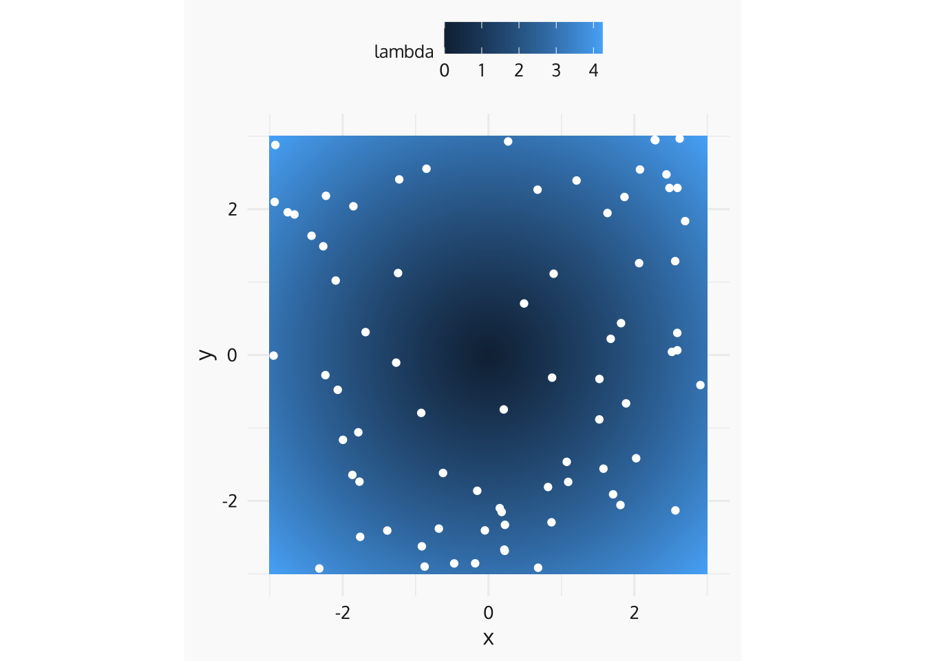
Special cases in 1 dimension
The Interval Specification
Define \(T_1 = X_i\) and \(T_i = X_i - X_{i-1}\) for \(i \geq 2\).
A homogeneous Poisson process has
\[\begin{equation*} T_i \overset{i.i.d.}{\sim} \text{Exp}(\lambda). \end{equation*}\]
An inhomogeneous Poisson process, the \(i^{\text{th}}\) inter-arrival time has pdf:
\[\begin{equation*} f_{T_i}( t \ | \ x_i) = \lambda(x_i + t)\exp \left\{ - \int_{x_i}^{x_i +t}\lambda(t)\mathrm{d}t\right\} \quad \text{ for } t \geq 0. \end{equation*}\]
The Counting Process Specification
Consider the cumulative number of points as a continuous time stochastic process.
- Highly dependent
- Exponential step lengths
- Almost surely unit step heights
n <- 20
T_i <- rexp(n)
X_i <- cumsum(T_i)
N_i <- seq(1, n)
t_min <- 0
t_max <- 1.1 * max(X_i)

x <- c(t_min, rep(X_i, each = 2), t_max)
y <- c(0, 0, rep(N_i, each = 2))
plot(
  x = x,
  y = y,
  xlim = c(t_min, t_max),
  ylim = c(0, 1.4 * n),
  type = "l",
  lwd = 1.5,
  bty = "n",
  xlab = "t",
  ylab = expression(N[t]))
Other Useful Properties
Superposition is like point process addition.
Random Thinning is like point process division.
Poisson processes are closed under superposition and random thinning. Can you prove this?
Areas for Further Exploration
Testing for CSR using these properties?
- difficulties with finite regions (edge effect corrections)
- complications for \(\lambda(t)\) non-constant (Ripley’s \(K\)-function)
How could these properties be used to simulate point patterns?
What happens if you relax some of these assumptions? E.g. Gamma inter-arrivals, points generated near existing points…