Workshop 4: Applications and Extensions

In this final workshop we will explore some of the areas in which Poisson processes are used. We will then consider a few of the ways that we might want to relax the strong modelling assumptions that are made by a Poisson process.

Extensions of Poisson Processes

So far we have focused exclusively on Poisson point processes

All events are treated the same
No co-incident points
Independence (and identical distribution) of inter-event times
Intensity function is deterministic

We can arrive at extensions of the Poisson process by considering different ways to relax each of these strong assumptions.

Marked and Multi-Type Point processes

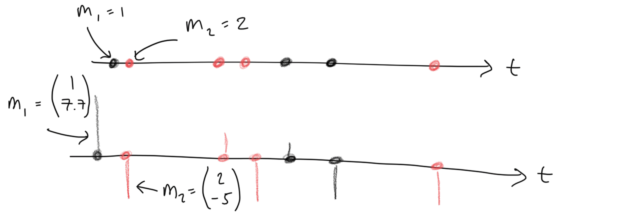
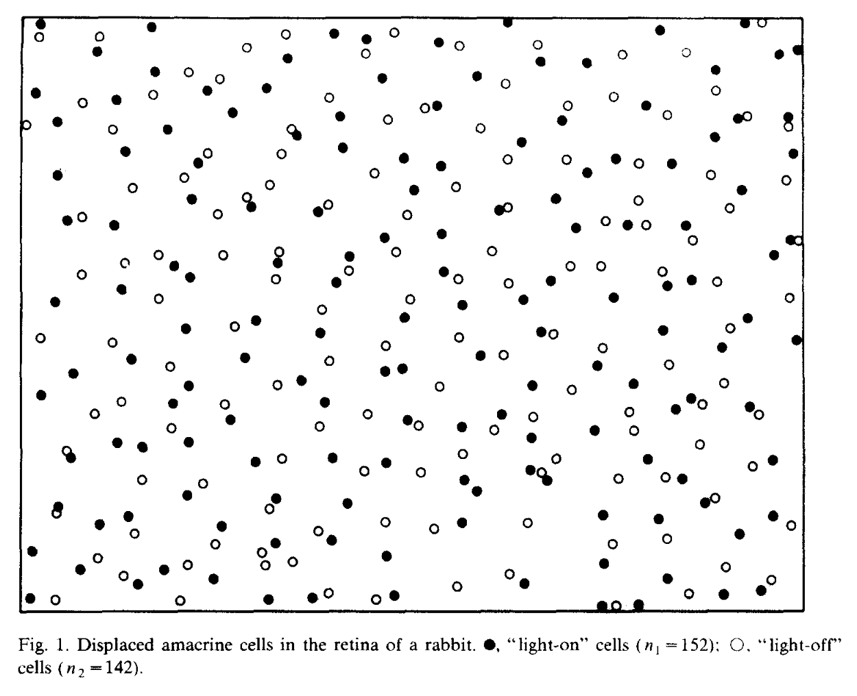
Marked Point Processes: Each event $x_i$ has associated covariate information $m_i$. This might be scalar- or vector- valued, stochastic or deterministic.

Multi-type Point Processes: are a special case, where marks are categorical random variables.

Example from Diggle (1986):

Non-orderly Point Processes

Through each of the specifications of a Poisson process, we ensured that the process was orderly: that there were no co-incident points.

\[ \lim_{\delta \rightarrow 0} \ \Pr (N(t, t + \delta)) = 0. \]

This need not apply generally. We can relax that assumption and have a mark $m_i )denoting the multiplicity of each event.

Renewal Processes

For homogeneous Poisson processes we have inter-event times are iid, independent and identically distributed.
Further, since these IETs are Exponential the waiting time from an arbitrary time has the same distribution.
The inhomogeneous Poisson process relaxes the identical distribution assumption by allowing the exponential parameter to change over space/time.
Renewal processes relax the identical distribution assumption beyond the Exponential distribution.

Interesting to study in 1D but the idea does not extend readily to other spaces. See, e.g. Cox and Isham (1980)

Adding dependence

We could also consider relaxing the independence assumption.

Allow the intensity of events $\lambda(t)$ to depend on the times (and/or marks) of previous events:

\[ \mathcal{H}_t = \{X_i \in X : X_i < t\}. \]

Most common examples of these are Markov point processes (See e.g. [Cox and Isham (1980)] and Hawkes (1970)) and Hawkes processes (Hawkes (1974)).

The former depends on $\mathcal{H}_t$ only through the most recent event(s), while the latter has a conditional intensity function of the form:

\[\lambda(t; \mathcal{H}_t) = \mu + \sum_{i:t_i < t} \alpha \exp\{-\beta(t-t_i)\}.\]

Compound Poisson Processes

We have seen (but not proved tat) superposition of independent Poisson processes remain a Poisson processes.

However, we can create much richer and more interesting structures within a point process by taking the superposition of dependent point processes.

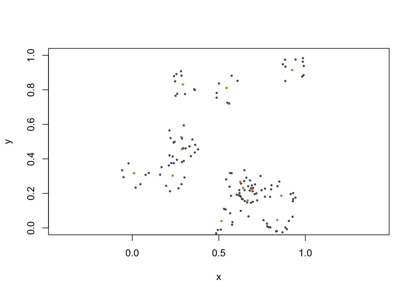
Many such interesting examples come from epidemiology, ecology or biology: e.g. first “generation” of cases HPP, secondary cases HPP on compact interval around first cases.

This generational perspective links some point process models to another class of stochastic process known as branching processes.

Adding another layer of randomness

Doubly Stochastic Point Processes do not have a fixed intensity function. The intensity is instead a random function.

We have actually seen an example of this already. The Hawkes Process is a doubly stochastic point process, because the value of the intensity function depends on the stochastic number and locations of events in the process.

This sort of history dependence is a sufficient way to construct a doubly stochastic point process but there are other ways too.

Log-Gaussian Cox processes link this back to the Gaussian processes we saw in the introductory lecture:

\[ \log \lambda(t) \sim \mathrm{GP}(\mu(t),\ K(\tau, \tau^\prime))\] These flexible models can be

Question: Do you remember why is the log needed here?

A word of warning: Simulation might be okay here if you use pre-packaged GP code, but avoid theory and inference for LGCPs.

Applications

Point process models are used widely in many areas:

Natural Hazards,
Finance,
Epidemiology,
Ecology,
Criminology,
Management and Operations Research.

A suitable project might be a review of Point process models in a particular application area with some corresponding theory or simulations.

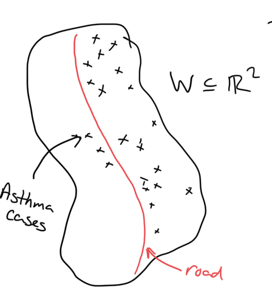
Point and Line Source Problems

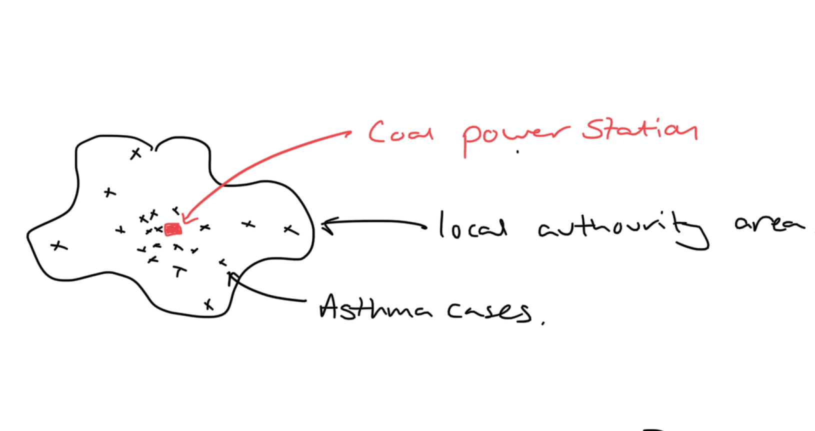
Point Source:

\[ \lambda(s) = \alpha \exp\{-\beta(s - s^*)\}.\]

Line Source:

We can consider our line source as a collection of point sources. We can then add the intensity contribution of each point source using a path integral:

\[ \lambda(s) = \int_{s^* \in L} \alpha(s^*) \exp\{\beta(s-s^*)\} \mathrm{d}s^*.\]

Queueing Models

Queueing sysems can be described in terms of Arrivals / Service / Servers.

Simplest version is $M / M / 1$.

$M$: Markov arrivals (HPP)
$M$: Markov service times (HPP)
$1$: Single server system

Generalised to $G/G/r$, similar to renewal processes.

Questions:

Theory: What is Campbell’s Theorem and how can it be used to help anmalyse such systems?
System perspective: What is the long-term behaviour of the system?
User perspective: What is the distribution of waiting times under different queue types?
Simulation: Can we establish this analytically or do we need to use simulation?
Inference: How can we use obsereved arrivals / service times to estimate the model parameters?

Advice

Start your poster now if you have not already.
Use or adapt a template, don’t start from scratch.
Sketch before you make.
Aim for a minimal working example.

Talk me through your idea / sketch. Do this today or book a 1-1 session on Teams next week. (Link to be added on Blackboard)